Hands-on dashboard tutorial · THERMA · About 25 minutes
A chiller can operate efficiently while the wider plant still uses more power than expected. Pumps and cooling towers matter, and an efficiency ratio is only useful when the power and cooling-load measurements describe the same boundary and period. This tutorial uses THERMA to connect three views of the plant: whole-plant efficiency, chilled-water temperature difference, and pumping power.
Your outcome: a short plant review with a checked kW/ton calculation, a correctly interpreted chilled-water delta T, and a documented pump-power contribution. You will observe the demo without changing staging, pump modes, or optimizer settings.
Before you begin
Open the THERMA browser demo and select Meridian Campus. Start on Plant Home. Readings are simulated and can move between observations. The examples below illustrate the method; they are not guaranteed operating results or recommended plant settings.
On a real installation, confirm what each power meter includes, how cooling load is calculated, and whether the readings share a timestamp. Check sensor quality and units. A dashboard makes the information easier to interpret, but the quality of the conclusion still depends on the underlying measurements and commissioning.
1. Capture one plant snapshot
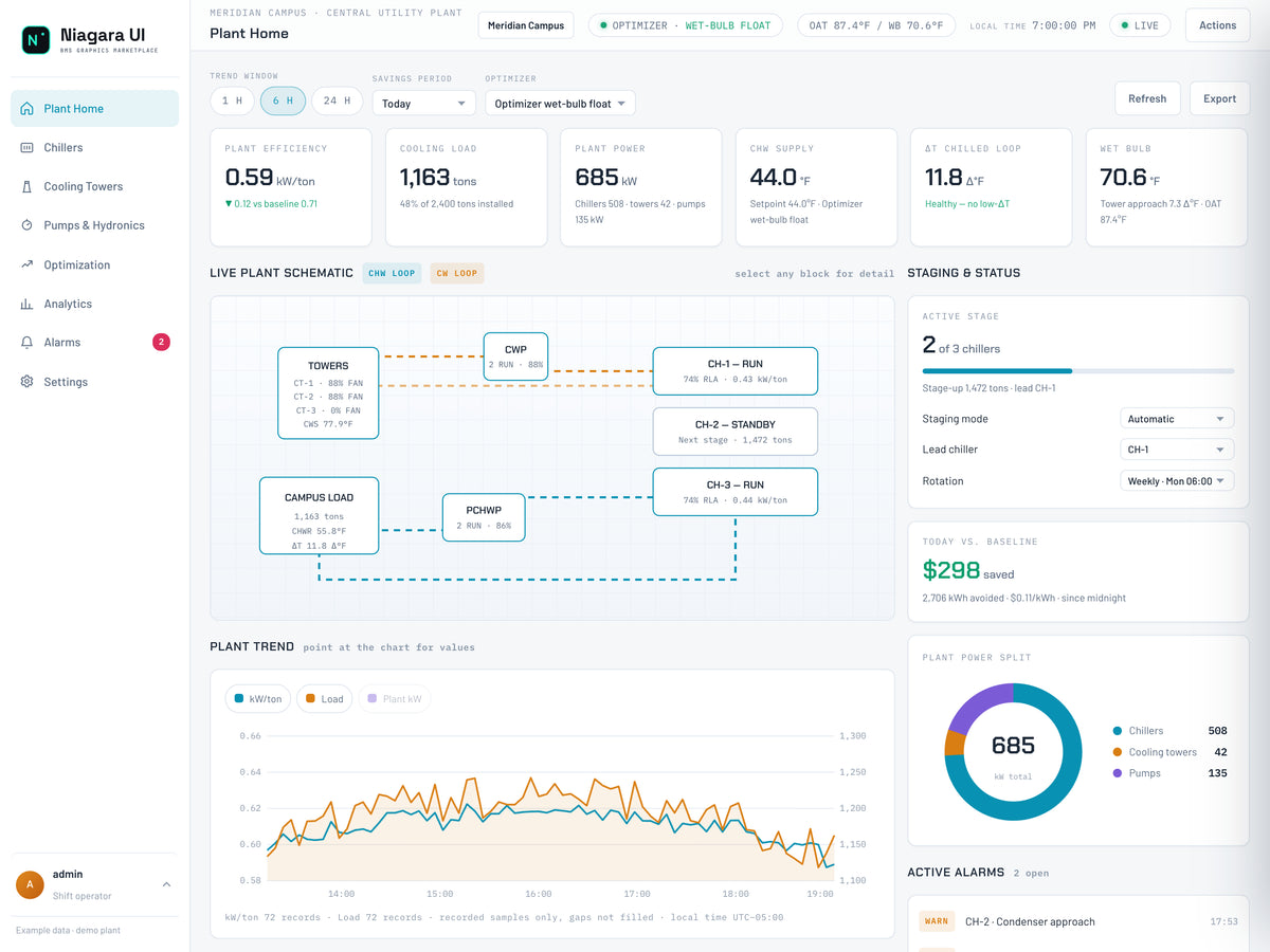
Read this screen
- Same-time snapshotRecord the selected plant, cooling load and electrical power with the same timestamp and units.
- Power boundaryWhole-plant power includes the configured chiller, tower and pump contributions.
- On Plant Home, record Plant Efficiency in kW/ton.
- Record Cooling Load in refrigeration tons and Plant Power in kW.
- Note the chiller, tower, and pump contributions shown in the power breakdown.
- Record chilled-water supply temperature, return temperature, delta T, and the observation time.
- Note the running chiller count and outside conditions to preserve the operating context.
A refrigeration ton is a rate of cooling, not a mass or an energy total. Likewise, kW is power at a point in time, while kWh is energy accumulated over time. Keeping these distinctions clear prevents comparisons that look plausible but do not measure the same thing.
2. Recalculate whole-plant kW/ton
Whole-plant kW/ton = included plant electrical power in kW ÷ delivered cooling load in tons.
In an example demo snapshot, Plant Power is 694 kW and Cooling Load is 1,150 tons. Dividing 694 by 1,150 gives approximately 0.604 kW/ton, consistent with a displayed value rounded to 0.60. The example power breakdown is 536 kW for chillers, 24 kW for towers, and 134 kW for pumps: 536 + 24 + 134 = 694 kW.
This check confirms math and the intended scope. It does not establish that the plant is optimally controlled. If your calculation differs from the displayed ratio, first check whether the readings refreshed at different times, whether rounding is involved, and whether the numerator includes the same equipment. Do not immediately attribute the difference to a plant fault.
Lower kW/ton generally means less electrical input per unit of cooling at the measured condition. However, compare like operating conditions: cooling load, weather, water temperatures, equipment availability, and metering boundaries all matter. A ratio at very low load can change sharply because the denominator is small.
3. Interpret chilled-water delta T
Find the chilled-water supply and return values in the plant schematic. For the cooling loop, use return temperature minus supply temperature. With return water at 56.4°F and supply water at 44.6°F, delta T is 11.8°F.
This is a temperature difference, not the supply-water setpoint. A plant can meet its supply-temperature target while the loop delta T differs from design. Compare the measured difference with the project's design intent and current load before calling it abnormal. There is no single correct delta T for every plant and every operating condition.
If delta T is unexpectedly low on a live project, possible investigation paths include sensor accuracy, bypass flow, coil performance, valve behavior, and load conditions. The dashboard reading identifies a question to investigate; it does not identify the cause by itself. Avoid changing flow or temperature targets solely to make the displayed number look better.
4. Open Pumps & Hydronics
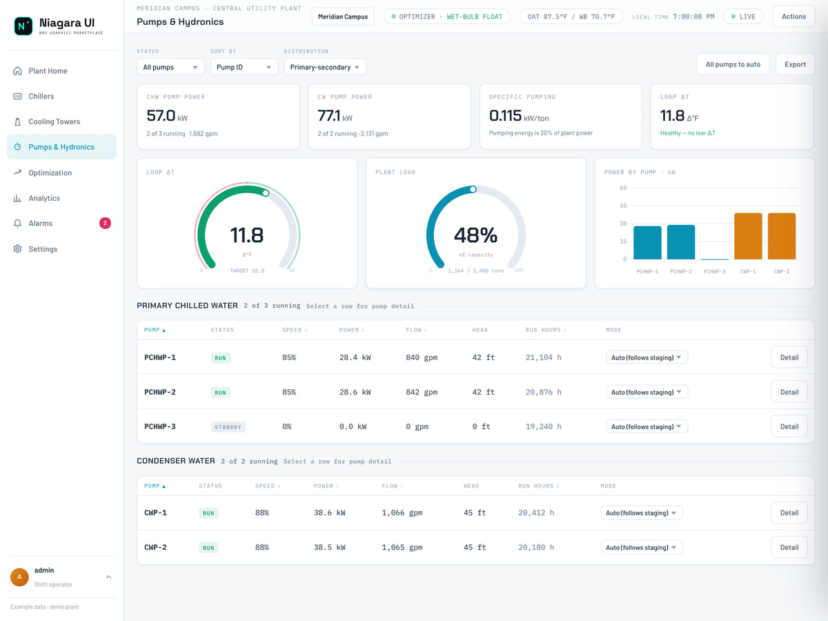
Read this screen
- Pump contributionInspect operating state and power alongside the plant load, rather than reading one pump in isolation.
- Hydronic contextRead entering/leaving temperatures, flow and delta-T together; record missing or unreliable inputs.
- Select Pumps & Hydronics in the navigation.
- Begin with All pumps so you can see both running and stopped equipment.
- Review chilled-water and condenser-water pump power, running counts, and flow summaries.
- Use the status filter to focus on Running pumps, and use the sort selector to compare Power or Run hours.
- Read the pump rows together: status, speed, power, flow, head, run hours, and mode.
Speed percentage is not a direct statement of power percentage or delivered flow. Compare the measured quantities and their units rather than assuming that a pump at half speed consumes half its rated power. Likewise, different pumps may serve different duties; a higher-power row is not automatically the least efficient pump.
5. Calculate the pumping contribution
The demo can show approximately 55.7 kW of chilled-water pumping and 77.9 kW of condenser-water pumping. Together that is 133.6 kW. Against 694 kW of plant power, the share is 133.6 ÷ 694 × 100, or about 19.3%.
To express the same contribution per unit of cooling, divide 133.6 kW by 1,150 tons: approximately 0.116 kW/ton. This is the pumping contribution, not the entire plant ratio. Small differences from the live demo card are expected when values refresh or are rounded.
For a real report, capture simultaneous readings and use a consistent equipment boundary. Do not combine a current pump total with a cooling-load reading from another hour. Also avoid double-counting a pump meter already included in an aggregate power point.
6. Review the trend before drawing a conclusion
Return to Plant Home. Use the available trend window controls and compare kW/ton, Load, and Plant kW. Look for whether a ratio change coincides with load or staging changes. Record the period being reviewed and any missing or questionable data.
The demo also shows baseline and savings information. Treat those as demonstration calculations, not a promise of savings. For a project-level savings claim, document the baseline method, comparable conditions, energy interval, tariff assumptions, and measurement boundary. A lower instantaneous ratio alone does not establish an annual financial result.
Completion checklist
- Power and cooling load captured for the same operating snapshot.
- Whole-plant kW/ton independently calculated.
- Chilled-water delta T calculated as return minus supply.
- Pump power separated from total plant power.
- Trend context and operating conditions recorded.
- Next verification stated without an unsupported optimization claim.
Explore the THERMA dashboard package, access Software Downloads, or request a demonstration to discuss your plant. A license is required to run the package on your host.